GPU-Accelerated Real-Time Passive Coherent Location: A Novel Parallel Shift-Correlate Approach
1. Introduction
Passive Coherent Location (PCL) radars constitute an alternative class of systems that do not emit their own signal. Instead, they use \textbf{transmitters of opportunity} (e.g., FM radio, DVB-T, GSM) for target detection. A key advantage of PCL is its undetectability and effectiveness against stealth technology. However, the requirement for high-throughput signal processing, especially when detecting slow-moving targets against strong ground clutter, necessitates advanced computational methods. Our core achievement is the development of a highly parallelized, GPU-accelerated algorithm to generate the Ambiguity Function (AF) map in real-time.
2. Mathematical Formalism of Ambiguity Map Calculations
The ability of any radar system to distinguish targets is characterized by the Ambiguity Function. We implement the Cross-Ambiguity Function (CAF) in the frequency domain using the Fast Fourier Transform (FFT).
2.1. Classical and Discrete Definitions of the CAF
The continuous form of the CAF \(\chi(\tau, f_d)\) measures the correlation between the reference signal \(x(t)\) and the tested signal \(y(t)\) shifted by a time delay \(\tau\) and a Doppler frequency \(f_d\):
For digital implementation, the discrete approximation (DCAF) is calculated over a Coherent Processing Interval (CPI) of \(N\) samples, where \(l\) is the discrete delay index and \(n\) is the discrete time index for summation:
2.2. Doppler Zoom Factor and Shift Value
To focus the analysis on specific, narrow bands of Doppler frequencies, a dynamic zoom factor \((z_f)\) is introduced. The required discrete shift value \(\Delta m\) for the frequency domain is calculated as:
Here, \(N\) is the FFT size, \(M\) is the number of Doppler columns, and \(Z=N/M\) is the unit zoom factor. The smaller the \(z_f\), the greater the Doppler magnification.
2.3. Core Frequency Domain Computation
Input signals are transformed into the frequency domain, where \(k\) is the frequency index \((k \in [0, N-1])\):
The core correlation, incorporating the cyclic Doppler shift, is performed via the element-wise product (Hadamard product) of the centered reference spectrum \(X[k]^{\Delta_{1/2}}\) and the cyclically shifted tested spectrum \(Y^*[k+\Delta m]\):
The final Ambiguity Map \(A[l, m]\) (range/delay and Doppler information) is obtained by performing the Inverse Fast Fourier Transform (IFFT) on the resulting matrix \(W[k, m]\) along the frequency dimension \(k\):
The index \(l\) in \(A[l, m]\) is the discrete delay index, consistent with the DCAF definition in (2).
3. GPU Acceleration and Segmented FFT Optimization
The overall algorithm execution is dominated by the FFT/IFFT steps. Our GPU implementation, utilizing CUDA/HIP libraries, leverages the {Fast Ambiguity Function (F-FAST)} method, which is based on the Convolution Theorem.
3.1. Segmented Forward FFT (Plan 1)
To overcome the memory and latency limitations associated with a single large DFT of length \(N\), we employ {Segmented Processing} (derived from Overlap-Add/Save principles). This optimization is applied to the generation of the conjugated DFT of the tested signal, \(Y^*[k]\), which is often the largest dataset.
The tested signal \(y[l]\) is divided into \(B\) independent segments, each of length \(N_{len}\). The total required conjugated test spectrum \(Y^{*}[k]\) is reconstructed from the segmented DFTs:
This method significantly reduces latency by replacing one large FFT operation with a batch of smaller, highly efficient ones, implemented using a batched cufftPlanMany (Plan 1).
3.2. Segmented Correlation and Reconstruction
The correlation in the frequency domain is performed by the CorrelateShiftCUDA kernel as a full \(N \times M\) operation. The final matrix \(W[k, m]\) uses the segment-reconstructed spectrum:
Crucially, the final Inverse FFT (Equation 7) is performed at the full length \(N\). This full-size IFFT ensures that the effects of the segmented forward transforms are correctly summed, maintaining the mathematical integrity and physical dimensions of the long-length correlation result \(A[l, m]\).
The GitHub code and binaries of Passive Radar for Windows 11 64bit is here.
The code for super fast ambiguity function FAF (NVIDIA CUDA) is here. The library supports one or two dongles. A more detailed description can be found here in pdf.
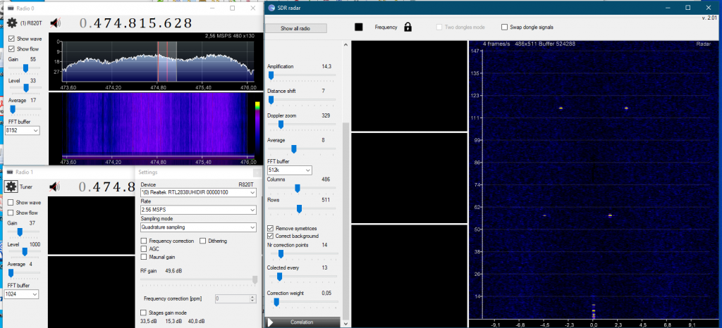
The Old passive radar in action
The resolution is 40×40 with around 70 frames/s of continous data flow! The RTL-SDR dongle does not have the best parameters, but analyzing 2097152 bits per frame gives interesitng results. The movie was recorded in a not the best location because the DVB-T transmitter (490MHz) was located on the right at 0.5 km and some buildings close to the road shadowed the signal. Cars give a negative doppler shift as they drive away. Arriving vehicles produce a positive doppler shift. The distance is around 50–300 m. The car’s speed is around 30–50 km/h. Each displayed frame is an average of 30 frames. The background is substracted and the left-right symetric filter is applied (substract the lower value from both pixels on left and right from the main 0 doppler shift line).
The link to the movie is here and here. Another exaple of this passive radar is a a video of the scattered signal from plane around 10km away (below).
Old PassiveRadar in action. The DVB-t tower is around 20km from my antenna. The DVB-t power is 56kW. The signal comes from a small sport plane (Cesna?) around 6-8 km from my place in the direction of DVB-t. The signal sometimes is below the line of trees because the plane has a low altitude of 1km.
Curently a new version of Radar 600% faster is available in Github. This version works togeter with improved code for Ambiguity function in repository it is AmbiguityUltra. Movie form this version of Radar is here.
With function remove symmetrices
New passive radar project
The new project consists of:
1) Radio with 4 passive radars that are tuned to the different DVB-t frequencies. The towers cannot lay on the same line!
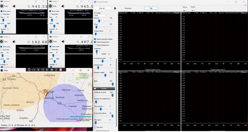
2) Signal translation to a list of time and Doppler shifts In digital form for each radar (a list of data). One bistatic radar can give more than one signal, e.g., other objects. The algorithm searches for blops on the screen (or array) and returns the middle of the blop (in radar as a geometrical center of mass center from the pixel value). The code is here. and the example is below. The red dots are the geometrical centers of the blops. The process is controlled by two arrays that are 'tested’ and 'found’. The heart of the algorithm is:
   for (int i = 0; i < blop_points.Count; i++)
       if (scaned_points[blop_points[i].X, blop_points[i].Y] == false)
           blop_points.AddRange(ScanNeighburst(blop_points[i]));
3) Mathematics to calculate the real position of the plane based on the position of 3 DVB-t towers. This is: observer position, 3 bistatic signals and DVB-t positions. It was a good math exercise; see figure below. To get the coordinates of point P(plain) in 3D you have to solve system of the presented equations (in color) with additional 9 pitagoras relations, which are not shown. The result has two solutions but only one with positive height over ground is the most interesting (done).
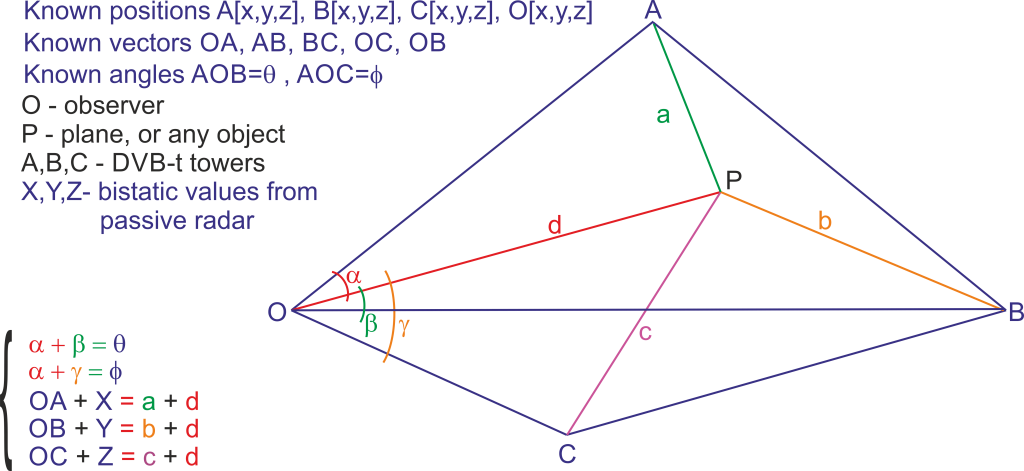
Below is the code that solves the problem for P. This problem can be reversed. O (observer) can be a position of DVB-t and A,B, C can be a position of observers. The math is exactly the same. With 4 computers connected to 4 different recivers it is possible to get exact position of point P. The smal inconvenience is the analysis of the data which have to be done on one computer or server. To do this every computer has to send its data with time stamp for every calculated frame. This is not that much data. Other option is to use two SVB-t towers with two computers (with recivers). And the work is as above, send calculated frames with time stamps to the server.
        static void CalculateDistance3(double OA, double OB, double OC, double X,
                                       double Y, double Z, ref Data dat)
        {
            //All geometry is in ECI (km)

            double S1, S2, S3, S4, S5, S6, S7, S8, S9, S10, S11, S12;

            S1 = (2.0 * OA * X + X * X);
            S2 = -2.0 * (OA + X);
            S3 = (2.0 * OB * Y + Y * Y);
            S4 = -2.0 * (OB + Y);
            S5 = (2.0 * OC * Z + Z * Z);
            S6 = -2.0 * (OC + Z);

            //Can be calculated once for given BTV positions
            S7 = Math.Cos(dat.teta);
            S8 = Math.Sin(dat.teta);
            S9 = Math.Cos(dat.phi);
            S10 = Math.Sin(dat.phi);

            S11 = OA / OB;
            S12 = OA / OC;

            double P1, P2, P3, P4;

            P1 = S11 / S8;
            P2 = S7 / S8;
            P3 = S12 / S10;
            P4 = S9 / S10;

            double P = P1 * S3 - P2 * S1 - P3 * S5 + P4 * S1;
            double Q = P3 * S6 - P4 * S2 + P2 * S2 - P1 * S4;

            // d is the  PO distance
            if (Q == 0) return; //just in case

            dat.d = P / Q;
            dat.a = OA + X - dat.d;
            dat.b = OB + Y - dat.d;
            dat.c = OC + Z - dat.d;

            double S1dS2 = S1 + dat.d * S2;

            //calculate alpha and dependent angles
            double N1 = S11 * (S3 + dat.d * S4) - S7 * S1dS2;
            double N2 = S8 * S1dS2;

            dat.alpha = Math.Atan2(N1, N2) + Math.PI;
            dat.beta = dat.teta - dat.alpha;
            dat.gamm = dat.phi - dat.alpha;


            double w = S1dS2 / OA / Math.Cos(dat.alpha);

            // only positive solution becouse over ground
            dat.h = Math.Sqrt(w * w / 4.0 + dat.d * dat.d);

            //ground vectors
            //a1=sqrt(a*a-h*h)
            //b1=sqrt(b*b-h*h)
            //c1=sqrt(c*c-h*h)
            //d1=sqrt(d*d-h*h)
        }
4) From the data obtained in step 3, the coordinates [x,y,z] of point P can be calculated from the intersection of three spheres (we know tower positions and the radii to the P (which is already calculated in step done).
5) because radars can detect more than one signal, it is necessary to receive a signal from the 4th DVB-T tover. In this case, all calculated positions must be compared to select only one correct solution (a plane position P). In this task, all possible combinations of detected signals from 4 recivers are compared. The corect solution is the one for which solution from recivers 1,2,3 and 1,2,4 gives the same spot. Additionally, this will give a position error.
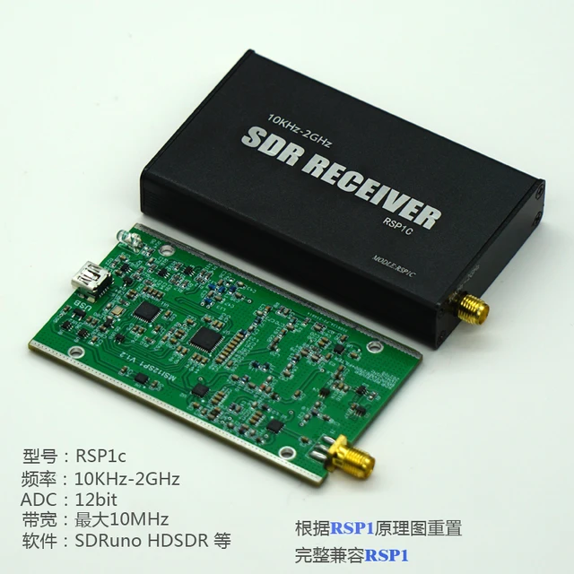
6) Ok , finally I completed the driver for the RSP1c and similar one. The driver is for Windows 10, 11. It supports the newest libusb.dll! The driver bases on the code of Miroslav Slugen and the addition of Leif Asbrink SM5BSZ. I hardly modified the code changing all the parts responsible for communication with windows. I also improved the bulk transfer and solved some issues with stability. I must say, the driver supports 99% of what I could find in Internet which is:
To use the new driver it is necesary to download the latest Radar2. This program suports the RSP1c dongle, RX888MK2 and one of the best AirSpy (my favorite).
Code of Radar2 which uses the RSP1c driver. This is the latest version of radar after meny modifications. It is much faster than the first version of Radar. The Ambiguity window with size 100×100 (rows x columns) with buffer size of 1024MB is refreshed more than 120 times/s with NVIDIA 3060 (laptop). With buffer size of 4048MB it is capable to detect walking people with calculation speed of 30 calculations/s. The window frames/s are calculated separatly from the ambiguity function. The code is optimised to not block komunication between threads (40% faster now). Please, use the 64bit version. 32bit is possible but you need all the libraries (*.dll) also to be 32bit. For compilation remove the security blocking from *.resx files!
The latest Ambiguity function (a bit faster)
Radar2 uses Bing maps so if you need a fully functional bing map you have to use a map key (later I will show how to do it). Radar2 uses 4 dongles at once. The third window is dedicated to RSP1 dongle. For tests only one dongle can be used. It is also a good tool to compare RTL-SDR with RSP1. I must say it is really better device. The code in action will be soon on Youtube:)