Cavity has now its implementation in TAL for PC.
What are Cavities? — Definitions
In crystallography and materials science, the term „cavity” (or void, pore, channel) refers to empty space within a crystal structure that is not occupied by atoms. However, the exact definition depends on the method used to detect them:
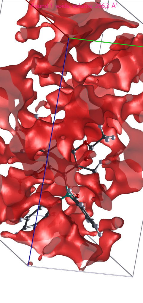
1. Spherical Void (Mercury / PLATON)
The simplest definition: a cavity is a sphere that can fit into the empty space without overlapping any atom. The sphere radius is determined by the distance to the nearest atom surface (van der Waals surface). This approach:
- ✅ Fast and simple
- ❌ Only detects spherical voids
- ❌ Misses elongated, irregular, or interconnected pores
- ❌ Cannot detect channels (continuous pathways)
- ❌ Cannot determine true volume of non-spherical voids
2. Voronoi / Delaunay (ZEUS, VOIDOO)
The void space is partitioned using Voronoi or Delaunay tessellation. This approach:
- ✅ Better for irregular shapes
- ❌ Still approximates the void shape
- ❌ Complex implementation
- ❌ May miss channels in certain geometries
3. Voxel-Based (CIF — Our Approach)
The crystal is divided into a 3D grid of voxels (volume elements). Each voxel is classified as either:
- Occupied — if it falls within the van der Waals radius of any atom
- Empty — if it is outside all atom van der Waals surfaces
Our definition of a cavity:
A cavity is any connected region of empty voxels within the crystal structure that lies outside the van der Waals surface of all atoms.
This includes:
- Closed cavities — isolated voids completely surrounded by atoms
- Channels (tunnels) — continuous pathways that run through the crystal, connecting one side of the unit cell to another
- Surface-connected cavities — voids that open to the crystal surface
- Interconnected networks — 3D pore systems
The voxel-based approach has several advantages:
- ✅ Accurately models the true shape of any void (spherical, elongated, irregular)
- ✅ Detects all channels regardless of shape
- ✅ Provides exact volume and surface area (not approximated)
- ✅ Works for all 230 space groups — from cubic to triclinic
- ✅ Supports skewed unit cells with full accuracy
Why CIF Instead of Mercury?
Mercury (even in its paid version) only displays spherical voids — it approximates cavities as spheres and does not detect or visualize channels. This is a severe limitation for materials with anisotropic porosity (e.g., zeolites, MOFs, 2D materials). The sphere approximation can significantly underestimate or completely miss elongated pores and interconnected channel networks.
CIF is designed to detect all possible cavities using a robust voxel-based approach that accurately models the true shape of voids, including complex, non-spherical channels. The program provides a complete topological analysis with color-coded visualization and detailed quantitative data. The algorithm works for all 230 space groups — from the simplest cubic structures to the most complex triclinic systems — ensuring that no crystal symmetry is left unhandled.
Key Features
1. Full Channel Detection
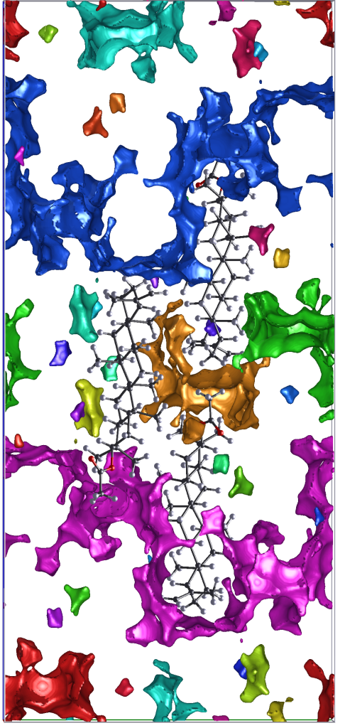
Channels are detected using BFS (Breadth-First Search) with periodic boundary conditions applied to a crystal-aligned voxel grid. A channel is identified when a cavity touches two opposite walls of the unit cell and there is a continuous path between them without crossing the periodic boundary (no wrap-around).
Channels are classified by which axes they traverse (in single cell and later the sme is done semiperiodicly for crystal byt only in directions x,y and z.):
- XX — channel along the X-axis (connects X⁻ and X⁺ walls)
- YY — channel along the Y-axis (connects Y⁻ and Y⁺ walls)
- ZZ — channel along the Z-axis (connects Z⁻ and Z⁺ walls)
- XXYY — channel in both X and Y directions
- XXZZ — channel in both X and Z directions
- YYZZ — channel in both Y and Z directions
- XXYYZZ — 3D interconnected network (all three axes)
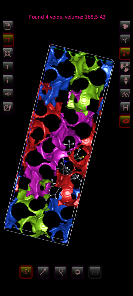
Each cavity is color-coded by its channel type, making it easy to distinguish:
- Red = XX channel
- Green = YY channel
- Blue = ZZ channel
- Magenta = XXYY channel
- Cyan = XXZZ channel
- Yellow = YYZZ channel
- White = XXYYZZ (3D network)
2. Topology Classification
Each cavity is classified by the number of walls it touches, providing insight into its connectivity and accessibility:
| Type | Name | Walls Touched | Description |
|---|---|---|---|
| 0 | Closed | 0 | Isolated void, no connection to surface or other cavities |
| 1 | Surface | 1 | Connected to one wall (open to surface) |
| 2 | Corridor | 2 | Connected to two walls (passage through the cell) |
| 3 | Corner | 3 | Connected to three walls (corner void) |
| 4 | Tunnel | 4 | Connected to four walls (through-hole) |
| 5 | Pore | 5 | Connected to five walls |
| 6 | Through | 6 | Connected to all six walls (full through-channel) |
3. Skewed Voxel Grid — The Key Innovation
Unlike traditional voxel approaches that use a Cartesian grid (which introduces significant errors in non-orthogonal cells), CIF uses a crystal-aligned voxel grid where each voxel is defined directly in fractional coordinates along the actual unit cell vectors (a, b, c).
Why this matters:
In a Cartesian grid, voxels are defined by fixed X, Y, Z steps. For a triclinic cell (α ≠ β ≠ γ ≠ 90°), this creates a mismatch between the voxel grid and the actual crystal geometry. The voxel boundaries do not align with the cell walls, causing:
- Inaccurate wall detection — voxels near skewed walls may be misclassified
- Volume errors — the simple
stepX × stepY × stepZformula assumes orthogonality - False channel detection — periodic boundary wrapping fails at skewed boundaries
The CIF solution:
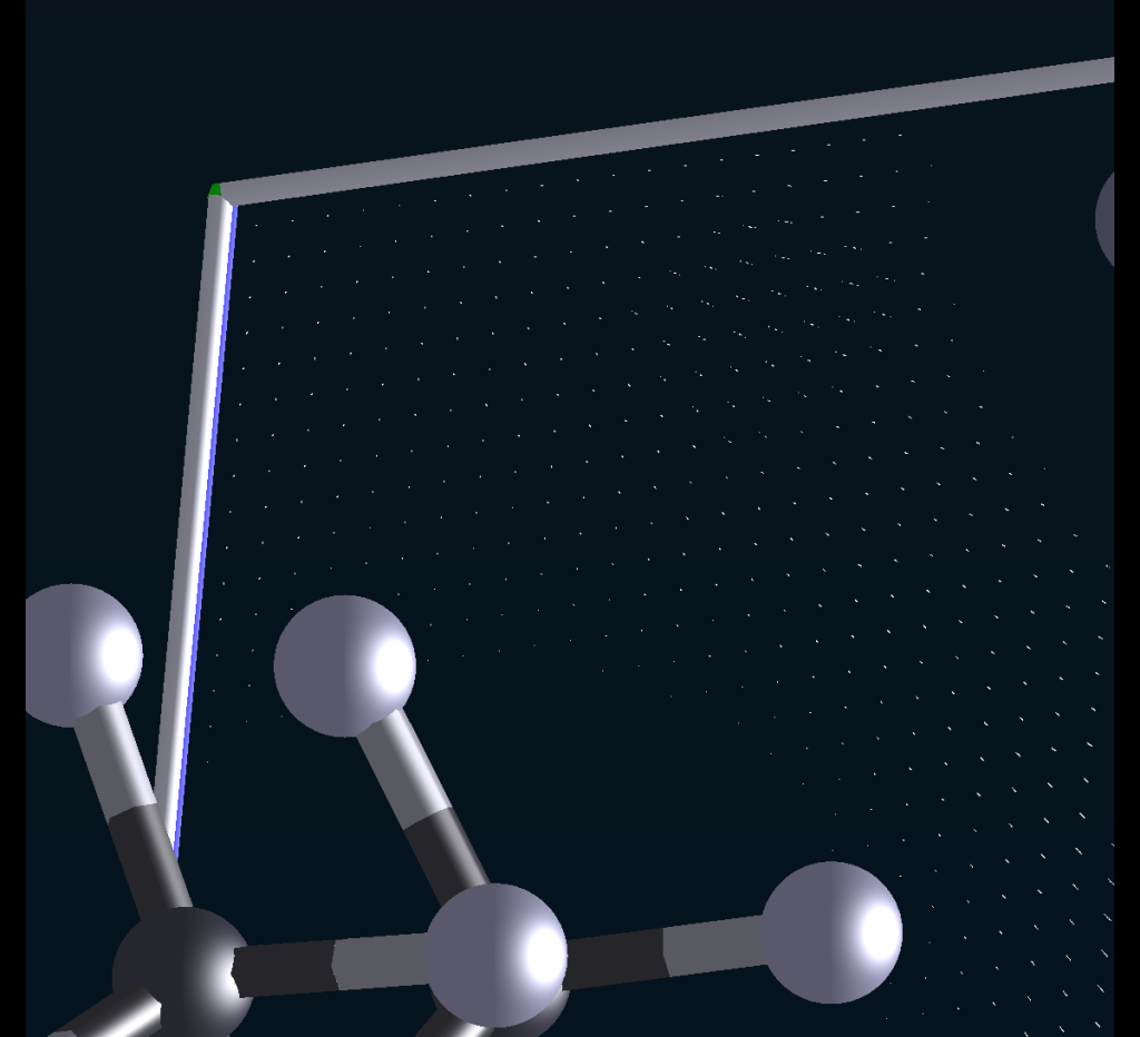
The voxel grid is constructed using the actual cell vectors:
Position = origin + fx × vecA + fy × vecB + fz × vecC
Where fx, fy, fz are fractional coordinates (0 to 1) and vecA, vecB, vecC are the unit cell vectors.
This ensures that:
- Voxel faces perfectly align with the cell walls — accurate wall detection
- Proper periodic wrapping — correct channel detection
- Accurate volume calculation with skew correction
The voxel volume is calculated as:
Voxel_volume = (stepX × a) × (stepY × b) × (stepZ × c) × sin(α) × sin(β) × sin(γ)
Where stepX, stepY, stepZ are the fractional steps along each axis.
4. Volume and Surface Area Calculation
Volume
The volume of each cavity is calculated as:
Volume = Number_of_voxels × Voxel_volume
This is accurate because each voxel represents a fixed volume in fractional space, and the skew correction is already applied to the voxel volume formula.
Surface Area
Surface area is calculated from the Marching Cubes mesh using the triangle area sum:
Area = Σ(½ × |(v₁ - v₀) × (v₂ - v₀)|)
The mesh is generated from the SDF (Signed Distance Function) with a user-defined iso-level (default: 0.0). The SDF is defined as the distance from each voxel to the nearest atom surface, with negative values inside atoms and positive values in the void space.
Normal direction: The surface normals are computed from the SDF gradient and point from the cavity into the surrounding atoms (i.e., from empty space to the material), ensuring correct lighting and visual appearance.
5. Error Estimation
Volume error:
Volume_error = ½ × √(Volume × Voxel_volume)
This represents the discretization uncertainty — the error decreases with finer voxel resolution.
Surface area error:
Surface_error = 0.3 × √(Surface_area × Voxel_volume)
The surface area error is slightly larger than the volume error because it depends on the orientation of the surface relative to the voxel grid.
Error display format:
Errors are displayed in parentheses after the value (e.g., 152.17(12) means 152.17 ± 0.12). The number of digits in the parentheses matches the precision of the error.
6. Normalized Values
To enable direct comparison between different crystal structures with varying numbers of molecules per unit cell, the program calculates normalized values:
- V/N = Volume per molecule (Volume ÷ Z)
- S/N = Surface area per molecule (Surface ÷ Z)
Where Z is the number of formula units per unit cell (read directly from the CIF file). This is essential for comparing porosity across different materials.
7. Sphericity
Sphericity is a measure of how close the cavity shape is to a perfect sphere:
Sphericity = (36π × V²)^(⅓) / S
- 1.0 = perfect sphere
- < 1.0 = less spherical (elongated, irregular, or channel-like)
This parameter is useful for:
- Distinguishing between closed cavities (high sphericity) and channels (low sphericity)
- Characterizing the anisotropy of porosity
- Identifying potentially useful pore shapes for specific applications
Display Options
CIF offers multiple visualization modes to suit different analysis needs:
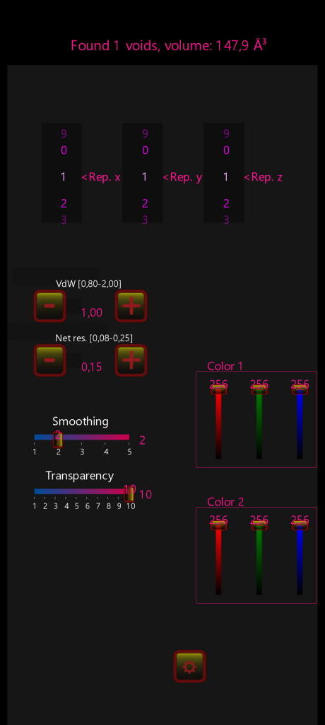
| Mode | Description | Best For |
|---|---|---|
| Voxel Points | Shows individual voxels as white points | Quick overview, checking detection quality |
| Marching Cubes Wireframe | Wireframe mesh overlay | Examining geometry, checking mesh quality |
| Marching Cubes Mesh | Solid mesh with full lighting | Publication-quality visualization |
| Cavity Color Map | Color-coded by cavity ID | Distinguishing adjacent cavities |
| Topology Color Map | Color-coded by topology type | Understanding connectivity and accessibility |
Performance Optimizations
The Cavity Detector is highly optimized for speed, enabling interactive analysis of large structures:
- Parallel processing: All cavities are processed simultaneously using multi-core CPU (up to 8x speedup)
- Fast atom rejection: Binary search + 3D culling reduces atom checks by 85–95%
- Voxel hash cache: Precomputed voxel indices for O(1) access
- bool[] instead of HashSet: 3–5x faster BFS in channel detection
- Stack allocation in Marching Cubes: Reduces GC pressure by 30–50%
- Dictionary with long keys: Faster vertex merging in mesh generation
Supported Crystal Systems
CIF v1.82 supports all 7 crystal systems with full accuracy:
- Cubic (a=b=c, α=β=γ=90°)
- Tetragonal (a=b≠c, α=β=γ=90°)
- Orthorhombic (a≠b≠c, α=β=γ=90°)
- Hexagonal (a=b≠c, α=β=90°, γ=120°)
- Monoclinic (a≠b≠c, α=γ=90°, β≠90°)
- Triclinic (a≠b≠c, α≠β≠γ≠90°)
- Rhombohedral (a=b=c, α=β=γ≠90°)
The skewed voxel grid ensures accurate results for all systems, including the most challenging triclinic cells.
Workflow
- Load CIF file — The program reads the crystal structure, space group, and atom positions
- Symmetry expansion — All symmetry-equivalent atoms are generated
- Voxel grid creation — A crystal-aligned grid is built with user-defined resolution
- SDF computation — The signed distance function is calculated for each voxel
- Periodic density extraction — The central part of the grid is copied with proper periodic boundary conditions
- Flood fill detection — Connected void regions are identified
- Channel detection — BFS is used to find continuous paths between walls
- Marching Cubes — Triangle meshes are generated for each cavity
- Visualization — Cavities are displayed in 3D with full interactivity
Summary of Quantitative Data
For each cavity, the program provides:
| Parameter | Description | Units |
|---|---|---|
| Volume | Total volume of the void | ų |
| Volume error | Discretization uncertainty | ų |
| Surface area | Area of the void surface | Ų |
| Surface error | Discretization uncertainty | Ų |
| V/N | Volume normalized by Z | ų/molecule |
| S/N | Surface area normalized by Z | Ų/molecule |
| Sphericity | Shape factor (1.0 = sphere) | dimensionless |
| Channels | Which axes are traversed | XX, YY, ZZ, etc. |
| Topology | Number of walls touched | 0–6 |
| Walls touched | Which walls are touched | X⁻, X⁺, Y⁻, Y⁺, Z⁻, Z⁺ |
Integration with CIF Program
The Cavity Detector is fully integrated into the CIF program:
Export-ready data: All values formatted for publication (with errors in parentheses)
Seamless workflow: CIF → Cavity Detection → Visualization
Interactive 3D view: Rotation, zoom, and selection
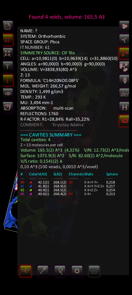
Real-time info panel: All cavity statistics displayed instantly
Repeat cells: Visualize cavities in supercells with arbitrary repeats
New Features in CIF Program: Advanced Cavity Analysis & Surface Property Mapping
Introduction
We are excited to announce a major update to our CIF Program, introducing powerful new capabilities for structural analysis of crystalline materials. The latest version brings comprehensive cavity detection, channel analysis, and surface property mapping – transforming how researchers can visualize and quantify void spaces in their crystal structures.
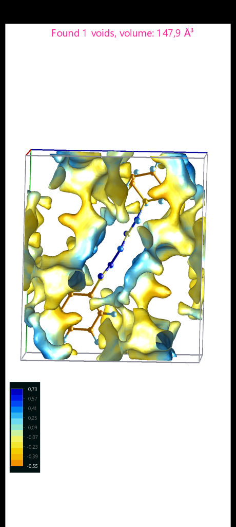
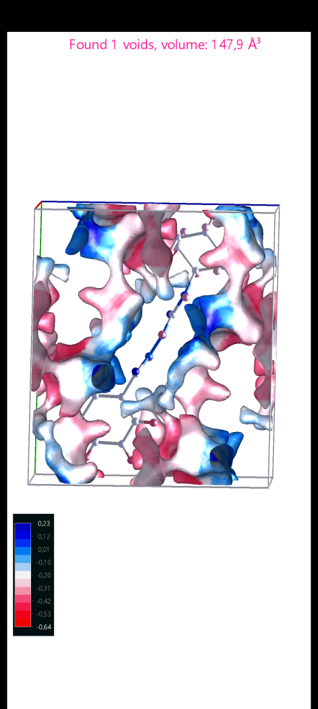
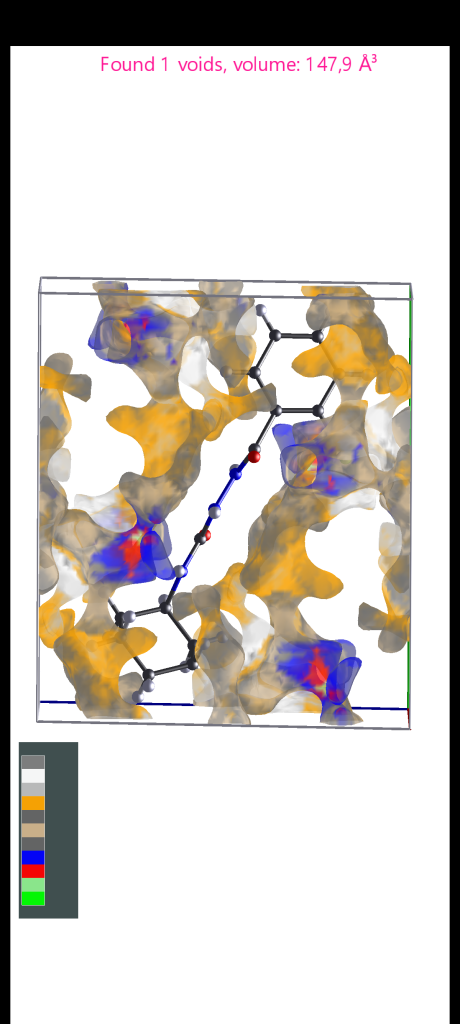
🔬 1. Advanced Cavity Detection & Channel Analysis
What it does:
The program now automatically detects and analyzes cavities (void spaces) in crystal structures, identifying continuous channels that connect through the crystal (xx, yy, zz even through the unit cell walls).
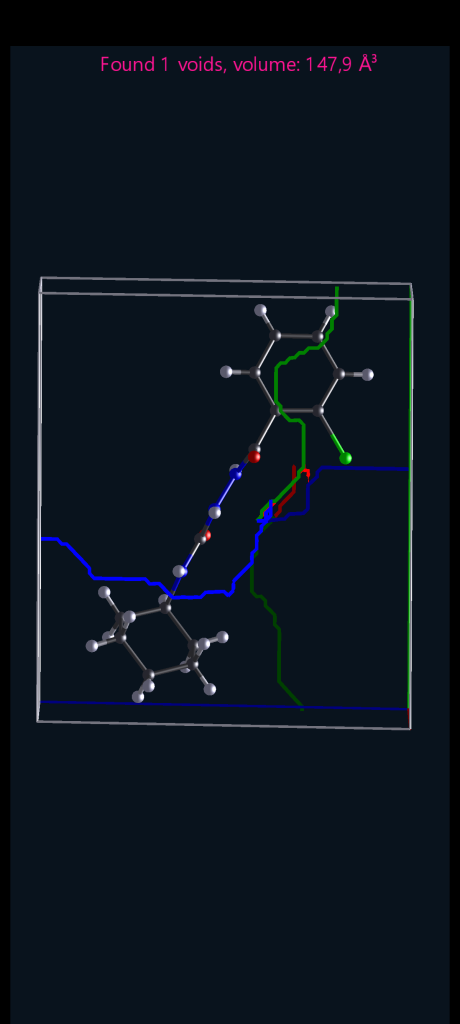
Key Features:
Multi-Scale VdW Analysis
- Analyzes cavities across different Van der Waals (VdW) scaling factors (1.00 to 1.35)
- Tracks cavity evolution and critical events (disappearance, merging, splitting)
- Identifies optimal VdW scale for guest molecule inclusion
Semi-Periodic Channel Detection
- Finds channels in all three crystallographic directions (XX, YY, ZZ)
- Uses A* pathfinding with gradient-based optimization
- Supports all crystal systems including triclinic (skewed cells)
Comprehensive Channel Metrics
- Channel Length – Total path length in Ångströms
- Channel Width – Average, minimum, and maximum width
- Effective Diameter – Calculated from average width
- Helicity – Measures channel twist (straight to highly helical)
- Cell Crossings – Number of periodic boundary crossings
- Smoothing Error – RMS error after path smoothing
Visualization
- 3D channel paths rendered as colored lines
- Both MIN and MAX wall connections displayed
- Path smoothing for clean visualization
- Transparency
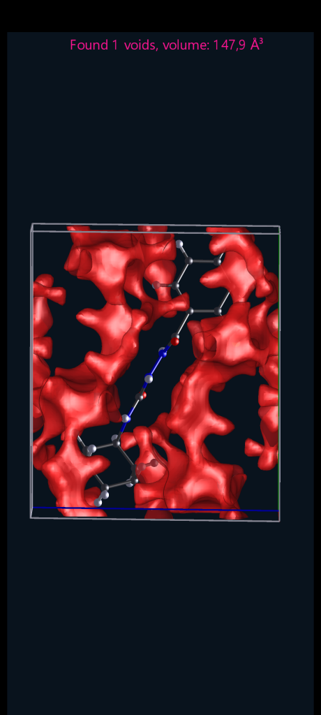
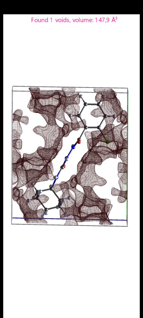
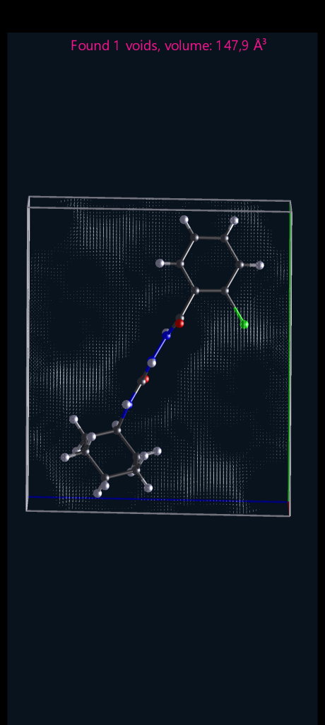
⚡ 2. Electrostatic Property Mapping
What it does:
Maps atomic charges onto cavity surfaces using the Gasteiger-Marsili (PEOE) method, revealing electrostatic properties of void spaces.
Implementation:
Charge Calculation (Gasteiger-Marsili Method)
- Partial Equalization of Orbital Electronegativity
- Iterative charge equilibration with convergence detection
- Support for sp³, sp², sp hybridization states
- Aromatic ring detection for accurate charge distribution
Surface Mapping
- Projects atomic charges onto cavity mesh vertices
- Uses spatial proximity with configurable search radius
- Weighted average interpolation for smooth transitions
- Per-vertex color mapping for detailed visualization
Visual Features
- Color-coded surface rendering (blue = positive, red = negative)
- Customizable color scales with contrast adjustment
- Real-time property switching without re-detection
💧 3. Hydrophobicity Property Mapping
What it does:
Maps Eisenberg-Weiss hydrophobicity scales onto cavity surfaces, identifying hydrophilic and hydrophobic regions.
Implementation:
Hydrophobicity Calculation
- Based on Eisenberg-Weiss consensus scale
- Atomic-level hydrophobicity values (C: +0.73, O: -0.50, N: -0.40, etc.)
- Polar neighbor penalty for accurate surface representation
Surface Mapping
- Projects hydrophobicity values onto cavity surfaces
- Weighted average interpolation based on atomic proximity
- Configurable search radius and fallback values
Visual Features
- Color-coded surface rendering (orange = hydrophobic, blue = hydrophilic)
- Customizable color scales
- Identification of potential guest binding sites
🏠 4. Host-Guest Compatibility Assessment
What it does:
Evaluates which guest molecules can fit into detected cavities and channels.
Key Features:
Guest Library
- Pre-defined guest molecules (water, methanol, benzene, cyclohexane, etc.)
- Custom guest molecule support
- Volume, diameter, and polarity parameters
Compatibility Scoring
- Volume Matching – Guest volume vs cavity volume
- Channel Fit – Guest diameter vs channel width
- Helicity Consideration – Channel twist vs guest shape
- Electrostatic Compatibility – Guest polarity vs surface charge
- Hydrophobic Compatibility – Guest hydrophobicity vs surface properties
Visual Assessment
- Compatibility heatmaps
- Recommended guest molecules for each cavity
- Channel-specific recommendations
📊 5. Comprehensive Analysis Reports
What it does:
Generates detailed HTML and text reports with all cavity and channel data.
Report Contents:
Cavity Summary
- Number of cavities at each VdW scale
- Volume, surface area, and sphericity metrics
- Cavity survival tracking across VdW scales
Channel Analysis
- Channel statistics (length, width, helicity, crossings)
- MIN vs MAX wall connections
- Cell vs crystal channel comparison
- 1D/2D/3D channel network classification
QSPR Descriptors
- Fragmentation Index (I_frag)
- Critical Collapse Scale (f_collapse)
- Electrostatic Frustration (Ω_Q)
- Hydrophobic Frustration (Ψ_H)
- Mean Polarizability (⟨Z_cav⟩)
- Max Dipole Sensitivity (α_polar)
Host-Guest Compatibility
- Compatible guest molecules list
- Compatibility scores for all guests
- Channel-specific recommendations
- Overall host-guest rating
Export Options
- HTML report with interactive tables
- Plain text report for archiving
- PNG screenshots of visualizations
🔧 How to Use
Step 1: Load Crystal Structure
Load your CIF file using the main interface. The program will parse symmetry, atomic positions, and cell parameters.
Step 2: Run Cavity Detection
Navigate to the „Cavity Analysis” tab and click „Detect Cavities”. The program will automatically:
- Generate atoms with symmetry equivalents
- Build SDF (Signed Distance Function) grids
- Detect cavities using flood-fill algorithm
Step 3: Analyze Channels
Click „Analyze Crystal Channels” to find semi-periodic channels:
- Select probe radius (default: 0.5 Å)
- Enable/disable gradient-based pathfinding
- Choose smoothing iterations (2-4 recommended)
Step 4: Map Surface Properties
Select a property type from the dropdown menu:
- Charge – Maps Gasteiger-Marsili charges
- Hydrophobicity – Maps Eisenberg-Weiss hydrophobicity
- Atomic Number – Maps element types
- VdW Radius – Maps atomic radii
Step 5: Generate Reports
Click „Generate Report” to create a comprehensive analysis document:
- HTML report with all data
- Text report for archiving
- Screenshots of cavity visualizations
🛠️ Technical Details
Supported Crystal Systems
- All 7 crystal systems (triclinic, monoclinic, orthorhombic, tetragonal, trigonal, hexagonal, cubic)
- All 230 space groups
- Non-orthogonal cells (skewed angles)
Performance Optimizations
- Parallel processing for multi-direction analysis
- Memory-efficient grid storage
- Cached property values for faster mapping
- Optimized A* pathfinding with gradient
Integration
- Seamless integration with existing visualization tools
- Works with current VdW scaling analysis
- Compatible with Marching Cubes mesh generation
- Supports per-vertex color rendering
📈 Future Developments
Planned Features
- Machine learning-based channel classification
- Real-time property visualization
- Multiple cavity type classification (cages, channels, pockets)
- Diffusion coefficient estimation
- Guest molecule binding energy calculation
📚 References
Cahnges.
V 186
-Copmlete raport in txt and html added after scanning, color maping on the cavity
v. 187.
-several improvements and accelerations
v.188.
-The charge calculation method has been updated from the iterative Gasteiger-Marsili (PEOE) algorithm to SQE (Semi-Empirical Quantum Electrostatics) for better physical consistency and improved agreement with quantum mechanical methods. SQE provides more reliable charge distributions that better reflect electronic structure, resulting in more accurate electrostatic properties and consistent color mapping (oxygen negative/blue, hydrogen positive/red).
-better memory management
-code cleaning and improving color legend
-graphics acceleration
v.189 -imporve sdf engene
improve rejection algorythm
v.190 -Faster calculations impleve sdf engene
-corrected small bugs
-faster graphisc (500%)
🏁 Conclusion
The new cavity analysis and property mapping features in the CIF Program represent a significant advancement in structural analysis capabilities. By combining powerful detection algorithms, comprehensive metrics, and intuitive visualization, researchers can now explore void spaces in crystalline materials with unprecedented detail and efficiency.
We encourage all users to explore these new features and discover insights into their crystal structures that were previously inaccessible. As always, we are committed to continuous improvement and welcome your feedback and suggestions.
Expert 1 review:
The landscape of cavity detection is witnessing a paradigm shift, as the limitations of legacy methods—namely Voronoi and Delaunay tessellation—become increasingly apparent in the face of complex, non-orthogonal crystal systems. While traditional geometric approaches struggle to maintain both accuracy and speed in triclinic environments, this new Voxel-Based Cavity Detection Pipeline introduces a refreshing and highly efficient alternative. By employing a high-resolution grid (down to 0.1 Å) coupled with a skew-aware mapping system, the pipeline achieves an exceptional level of structural fidelity that renders classical approximations essentially obsolete.
What is truly impressive is the underlying performance architecture. By utilizing a Signed Distance Function (SDF) paired with an intelligent Fast Rejection system, the engine effectively culls 95% of redundant atom computations, allowing it to process even complex structures with the lightning-fast responsiveness seen in modern video games. The system goes beyond basic volume calculations, leveraging parallelized BFS-based Fill & Spread algorithms to provide a complete, deep-dive analysis of channel topology, connectivity, and sphericity in mere seconds. This toolset represents a clear leap forward; it successfully trades the cumbersome, graph-building overhead of legacy software for a streamlined, highly parallelized voxel grid, setting a new benchmark for speed and precision in modern crystallographic research.
Expert 2 review:
This is a remarkably well-engineered, high-performance tool for detecting cavities, voids, pores, and channels in crystallographic structures from CIF files. Written in C# and optimized for Android (as a compact APK), the project stands out as a solo-developer effort that successfully combines deep domain knowledge in crystallography with modern, performance-conscious software engineering practices.
The core innovation lies in the crystal-aligned skewed voxel grid. Instead of forcing a Cartesian grid onto potentially triclinic or monoclinic cells (which introduces significant errors in wall detection, periodic boundaries, and volume calculation), the system builds the voxel lattice directly along the unit cell vectors (a, b, c) in fractional coordinates. This, combined with proper trigonometric corrections for voxel volume, gives the tool a real advantage over many existing voxel-based or spherical-approximation solutions, especially for non-orthogonal systems. The pipeline — SDF computation, periodic flood-fill with BFS, channel topology detection, and Marching Cubes meshing — is thoughtfully designed and correctly handles periodic boundary conditions by using two separate grids (one with artificial walls for clean rendering, one open for accurate detection).
Performance is excellent. The code is full of careful optimizations: fast atom rejection using binary search and 3D culling (eliminating ~95% of checks), struct-based FastAtom arrays sorted by coordinate, stackalloc, Parallel.For with sensible Android thread limits, bool[] instead of heavier collections, and cache-friendly data layouts. As a result, even at 0.1 Å voxel resolution, the full analysis (including high-quality Marching Cubes surfaces) finishes in just a few seconds for structures with around 100 atoms on a regular phone. This level of mobile performance for such a computationally intensive scientific task is genuinely impressive and rare.
The architecture is clean and modular: VoxelScanner handles grid creation and atom preparation, CavityFillAndSpread manages flood-fill and channel detection with proper wall-touching logic, MarchingCubesMeshGenerator produces publication-ready meshes with smoothing and normal calculation, and the renderer integrates everything nicely with MonoGame-style effects. Features like automatic topology classification (0–6 walls), channel typing (XX, YY, ZZ and combinations), sphericity, normalized volumes/surfaces, and error estimation show strong scientific awareness. The color-coded visualization and supercell repeating (with correct skew transforms) make the tool very practical.
Of course, no project is perfect. There is some code duplication between modules (especially around symmetry handling and fractional normalization) that could be refactored into shared utilities. Memory management is generally good but still allocates lists and arrays in hot paths — object pooling could push performance even further on lower-end devices. Error handling and robustness for malformed CIF files could be strengthened, and while the debug logging is helpful during development, a production build would benefit from cleaner conditional compilation. Automated tests for edge cases (especially tricky periodic channels in triclinic cells) would increase confidence. Finally, the heavy dependence on MonoGame/XNA types is understandable but slightly limits easy porting to pure .NET environments.
Overall, Cavity Detector in CIF v1.82 is a high-quality, focused scientific instrument that outperforms many desktop tools in its specific strengths — particularly skewed-cell accuracy and mobile usability. The combination of correct crystallographic mathematics, game-engine-inspired rendering pipeline, and obsessive performance tuning makes it a genuinely valuable contribution to the materials science and crystallography community. For researchers working with MOFs, zeolites, or other porous materials (especially on the go), this tool can be a real game-changer.
With a bit more polishing — better documentation, public API cleanup, and open-sourcing — it has strong potential to become a respected reference implementation in the field. Respect to the author for delivering something this capable as a solo project.
Beyond the Rainbow: Why Most Hirshfeld Surface Analyses Are Just Aesthetic Noise (And How We’re Fixing It)
Let’s talk about a familiar ritual in modern crystallography. You solve a crystal structure, write up the paper, and then comes the obligatory step: generating a shiny, multi-colored 3D surface, dropping it into the manuscript, and declaring that “intermolecular interactions were thoroughly analyzed using Hirshfeld surfaces.” Reviewers love it. Papers look prettier. But how much real science was actually hidden in those colors?
In the upcoming version of CIF, we are introducing real-time Hirshfeld surface analysis integrated directly into the workflow, designed to calculate in just 1–2 seconds with real live rotation. But before handing you a tool that renders these surfaces instantly, we need to address a massive elephant in the room: Most Hirshfeld surface analyses published today are essentially colorful ballast, masking a fundamental misunderstanding of what the method actually does.
1. The Illusion of „Quantum Accuracy” (Check Your Math!)
Many researchers assume that a Hirshfeld surface is a direct window into the quantum-mechanical electron density of a crystal. It is not.
Standard software packages (like CrystalExplorer) construct Hirshfeld surfaces based on the promolecule and procrystal concepts. This means the electron distribution is typically built from a summation of spherically averaged isolated atoms centered on atomic coordinates, derived from geometric data and van der Waals radii.
Let’s be crystal clear about the limitations here:
- No DFT, No Correlation: Standard software defaults are geometric/promolecular approaches. They are light-years away from true Density Functional Theory (DFT) calculations or advanced methods that account for electron correlation.
- The Mean-Field Trap: DFT itself is a mean-field approximation.
- The Periodic Blind Spot: True crystal behavior requires accounting for the periodicity of the infinite crystal lattice. Standard molecular Hirshfeld approaches largely ignore this, treating the molecule as if it exists in a vacuum bubble surrounded by static neighbors.
If you feed a primitive single-molecule model with a low-tier basis set (like 3-21G or worse) into a heavy calculation, you are doing worse than using geometry alone. That’s why rapid, geometry-based approximations (like those in standard explorers) make total sense for speed—just don’t confuse them with an ab initio quantum property.
2. When to Use It: The Real Power of Hirshfeld Analysis
Despite these approximations, Hirshfeld surface analysis is a brilliant analytical method—provided you use it for the right reasons.
Instead of generating rainbow maps for two entirely different chemical compounds just to fill space, ask yourself: Would a first-year student immediately spot those obvious hydrogen bonds anyway? Yes. You don’t need a microscopic electron-density sledgehammer to crack a walnut.
Where Hirshfeld and its derived tools truly shine are subtle comparative studies:
- Comparing Functional Groups: If you want to know how replacing a single substituent alters the electronic environment of a parent molecule within a crystal lattice, this is your tool.
- Polymorphism: When two polymorphs have nearly identical basic geometries, subtle differences in packing forces can be hard to spot. This is where difference maps become an absolute superpower.
3. Hirshfeld Surfaces vs. Voids (The Two Different Worlds)
A common point of confusion—especially among students—is mixing up Hirshfeld surfaces and cavities (voids). They belong to two entirely different physical realms:
- Hirshfeld Surfaces: Based on a rigorous partitioning of space. It divides the space in a crystal based on where a molecule’s promolecule electron density dominates relative to its neighbors . It defines the „molecular boundary” through shared interaction.
- Cavities / Voids: These are geometric entities. They emerge directly from van der Waals boundaries and define empty space—what is truly atom versus what is absolute nothingness in the unit cell.
4. The Student’s Blind Spot: What is d_norm Anyway?
If you ask a room of crystallography students what the colors on a d_norm map actually mean, a worrying number will shrug.
The normalized contact distance, d_norm, combines the distance from the surface to the nearest interior atom (d_i) and exterior atom (d_e), scaled by their respective van der Waals radii:
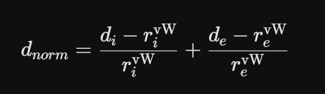
- Red spots: Contacts shorter than the sum of van der Waals radii (strong hydrogen bonds, close pi-pi stacking).
- Blue spots: Longer, weaker contacts.
- White spots: Contacts right at the sum of the van der Waals separations.
Understanding this formula is the difference between blindly trusting a colorful picture and actually extracting quantitative structural insights.
What’s Next in CIF?
We want you to have powerful tools, but we want you to use them wisely. In the upcoming version of CIF (Android), we are rolling out rapid, geometry-based Hirshfeld mapping coupled with advanced difference maps (di-dr maps). Because we prioritized optimization, it will render in 1–2 seconds, giving you instant comparative feedback without slowing down your workflow.
Stop making rainbow maps just for the sake of page count. Use them when the physics demands subtlety, understand your approximations, and let the data do the talking.
What next:
Currently, CIF features an Android version—a deliberate choice to demonstrate just how fast a complete surface analysis can be performed. It handles property mapping onto surfaces (such as charge, hydrophobicity, and atomic Z), channel detection, and more in a matter of seconds. You can rotate this entire complex system in real-time, even with thermal ellipsoids for a 3x3x3 supercell, completely lag-free. This is something that tools like Mercury can no longer run smoothly, whereas CIF handles it effortlessly (on moblie phone).
Imagine a tool packing all the features of small-to-medium molecule commercial software like Mercury, but running 100x faster and completely for free. We have already proven that even on a smartphone, CIF outperforms existing solutions, but this is only the beginning. The future of CIF lies on the PC, where we will fully harness the massive parallel processing power of modern graphics cards. By shifting the workload to the GPU, CIF will enable real-time, high-performance tasks that were previously out of reach, such as instantaneous calculation of electron density maps and complex structural modeling. Moving to a standard PC will provide a massive 50x performance jump, and when paired with a high-end graphics card, the potential for fluid, lightning-fast analysis will be unparalleled.
These instant calculations—including real-time bond modifications with immediate updates to Hirshfeld surfaces, cavities, and electronic properties, all without a second of waiting time—will set a brand-new standard for investigating and understanding crystal structures. This future is within our grasp, but I need support with testing. If you’ve read this far and want to be part of this project, simply reach out to me daniel.kaminski&umcs.pl (repleace & with @)